Angular & AI Meetup Graz · 11th September 2026
Developing withLocal LLMs: Reality or Illusion?
Welcome everyone and introduce the subject: this is not a session about replacing frontier models at all costs. It is about understanding what we gain, what we give up, and how an engineering system can make a local model useful for serious software work. The talk follows one practical question: can a model running on hardware we control implement a real full-stack feature and prove that it works? Keep the opening concise. Transition: before discussing models, define why an organization might care where inference happens.
Cover image: Angular Meetup Graz, https://secure.meetupstatic.com/photos/event/5/0/4/6/clean_524960550.webp .
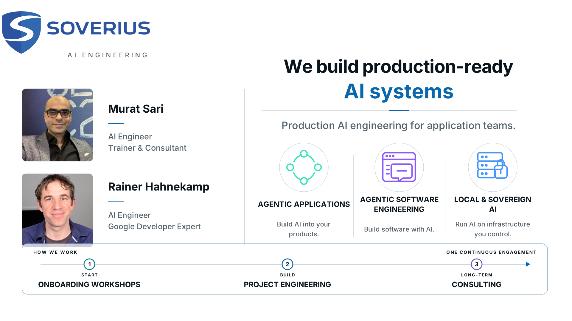
Introduce Rainer, Murat and Soverius AI briefly. Soverius is positioned as production AI engineering for application teams. Its three connected pillars are Agentic Applications, Agentic Software Engineering and Local & Sovereign AI.
The service path can begin with an onboarding workshop. Project engineering is where we build the system together with the customer team. Consulting can continue after delivery as long-term support. Customers can use one part or work with us across the complete path.
This talk connects Local & Sovereign AI with Agentic Software Engineering: it asks whether local models can perform serious software work and which engineering controls make that practical. Keep this introduction under ninety seconds. Transition: give the audience the four-part agenda for the webinar.
Agenda
LOCAL MODELS
FOR AI-ASSISTED
CODING
01
WHY
Why local models?
02
HOW
llama.cpp + Gemma 4
03
SHOW
Capstone
04
CHALLENGES
Speed and quality
SPEED
Hardware requirements
QUALITY
Loop / graph engineering
3
Introduce the four-part path. First ask why organizations consider local models. Then show how the local coding setup works with llama.cpp and Gemma 4. The capstone demonstrates the complete setup on a serious full-stack task. Finally, discuss the two practical challenges: speed through hardware requirements, and quality through evaluation, control loops and engineering around the model. Transition: begin with the reasons for running models locally.
Why Local Models?
LOCAL MODELS
FOR AI-ASSISTED
CODING
01
WHY
Why local models?
02
HOW
llama.cpp + Gemma 4
03
SHOW
Capstone
04
CHALLENGES
Speed and quality
SPEED
Hardware requirements
QUALITY
Loop / graph engineering
4
Open the first chapter. We begin with the practical reasons for running a model locally: cost control, privacy and independence.
Why local?
Reasons to Run Models Locally € Cost Control No provider charge per token.
Privacy Keep code and context inside.
Independence Reduce provider dependency.
5
The three main reasons are cost control, privacy and independence. Once the hardware is available, each additional local token has no provider charge. That does not make local inference free: hardware, electricity, operations and engineering time remain real costs. Local inference can keep source code, prompts, intermediate outputs and retrieved context inside a boundary controlled by the organization. It also reduces dependence on an external provider and on changes to external terms, availability or model versions. Transition: show the components required for our local coding setup.
Icon source: Lucide, https://lucide.dev/ (ISC license).
Setup and Configuration
LOCAL MODELS
FOR AI-ASSISTED
CODING
01
WHY
Why local models?
02
HOW
llama.cpp + Gemma 4
03
SHOW
Capstone
04
CHALLENGES
Speed and quality
SPEED
Hardware requirements
QUALITY
Loop / graph engineering
6
Open the setup chapter. Introduce the three required components, then move directly into the live demonstration.
Local Inference Demo 8
Demo goal: remove the mystery, not prove the benchmark. Show the inference process already running, the model loaded, and the local endpoint. Send a small repository question through the coding agent and point out the three boundaries: the agent sends a prompt, llama.cpp performs inference, and the model returns tokens. Prepare a recording or screenshots in case live loading takes too long. Do not use the capstone as the first demo. A short read-only question is enough. Transition: with the local setup now concrete, use the capstone to show a complete full-stack task.
The Capstone
LOCAL MODELS
FOR AI-ASSISTED
CODING
01
WHY
Why local models?
02
HOW
llama.cpp + Gemma 4
03
SHOW
Capstone
04
CHALLENGES
Speed and quality
SPEED
Hardware requirements
QUALITY
Loop / graph engineering
9
Return to the map and highlight Show. Before presenting the capstone, define how we evaluate the model: make the trade-off between quality and data sovereignty explicit, use the Porsche analogy to question whether every task needs peak capability, and set the qualification bar. Then show the task used to test that bar.
Quality vs Data Sovereignty
Data Sovereignty
Quality
Local Models
High Quality Data Sovereignty Frontier Models
Peak Quality No Full Data Sovereignty
Speed is a hardware budget question. Powerful local hardware can match cloud inference speed.
10
Treat these as two qualitative positions, not measured data points. Local models can deliver high-quality software work while keeping model execution and data inside infrastructure the organization controls. Frontier models still provide peak capability, but closed provider-hosted models do not provide full data sovereignty under this definition. Contracts, regional hosting and technical controls can improve privacy and governance, but the organization does not control the complete inference stack. The bubbles deliberately avoid precise coordinates because individual models, tasks and deployment choices vary. Treat speed as a separate question. Local inference speed mainly depends on hardware capacity and budget. With sufficiently powerful accelerators and a comparable model configuration, a local system can match the latency or throughput of cloud inference. Transition: use the Porsche analogy to ask whether every software task needs peak model capability.
The Porsche test
Do We Need Peak Capability for Every Trip? Most software tasks never reach the empty, unrestricted Autobahn.
Use the car as an analogy, not a proof. A sports car can deliver extraordinary speed, but most trips never encounter an empty, unrestricted Autobahn. Selecting every system for the rare theoretical maximum can be wasteful if everyday work has a lower, well-defined requirement. Software tasks vary enormously. Some genuinely need the strongest available model: novel debugging, unclear requirements or discovery across a large repository. Many routine changes are narrower and easier to verify. The question becomes: which model reliably clears the bar for our work? Transition: define that bar.
Benchmark philosophy
Qualification Instead of Ranking Qualification threshold
Model A
Model B
Model C
Qualification criteria ✓ Works with coding agents
✓ Handles long-running tasks
✓ At least 128K tokens of context
12
We are not building a universal leaderboard. We define tasks that represent our work and a bar that represents acceptable completion. Every model that repeatedly clears the bar becomes a candidate. For this webinar, serious software work means that the model works with a coding agent, can remain effective during long-running tasks, and provides a context window of at least 128K tokens. That context has to hold repository information, instructions, loaded skills, tool results and verification evidence. The 128K figure is our practical minimum, not a universal standard. Benchmark results still depend on the runtime, agent and workflow, which we cover later. A single success is evidence, not a timeless property of a model. Transition: apply the qualification bar to the capstone task.
The Capstone
Full-Stack Capstone Task Angular Feature component UI component SignalStore Unit test Spring JPA entities Mapper Controller Database migration Playwright 13
The capstone is deliberately broad and delivered as one prompt. On the Angular side, the model must implement the feature according to existing architecture, separate feature and UI responsibilities, use a SignalStore, and add tests. On the Spring side, it must add the JPA model, mapper, controller and database migration. Finally, it must add a Playwright end-to-end test. This is difficult because success requires repository discovery, architectural consistency, cross-boundary changes and verification—not because one file is exotic. Logo sources: https://simpleicons.org/?q=angular, https://simpleicons.org/?q=spring, https://playwright.dev/img/playwright-logo.svg. Transition: show the exact one-prompt specification used for the capstone.
The Capstone Prompt
/goal

In my holidays overview I want a German vocabulary trainer, similar to the existing quiz feature. For destinations in German-speaking places (currently Lübeck and Vienna) users should be able to practice a few basic German words before they travel: the holiday card shows an icon when a vocabulary test is available, and opening it lets the user translate words.

Do a full-stack implementation (backend + frontend) following the structure and conventions of the existing quiz feature (architecture, feat folder, backend entity/repository/controller). The app must be accessible, and the accessible names below are required. Create and run e2e tests for the feature.

Acceptance Criteria

1 Successful Verification
- The frontend build check is pnpm ng build --optimization false.
- Start any required application dependencies using the project's existing setup, then start the backend with ./gradlew bootRun.
- Wait for the backend to become ready and verify that both the existing /heartbeat and /holiday endpoints respond successfully. Starting the process alone is not sufficient.
- Start the frontend on port 4200 and run the vocabulary feature's e2e tests with the project's Playwright setup.
- If compilation, application startup, an endpoint request, or an e2e test fails, diagnose the failure, fix the implementation, and repeat the relevant checks. Do not finish while a required check is failing.
- Stop all application processes and temporary services that you started after verification, including when a check fails.

2 Vocabulary Data
- A vocabulary test consists of exactly 5 words. Each is an English word the user must translate into German.
- Use exactly these 5 English -> German pairs, stored verbatim (capitalization and umlauts matter):
  squirrel      -> Eichhörnchen
  turtle        -> Schildkröte
  refrigerator  -> Kühlschrank
  toothbrush    -> Zahnbürste
  Germany       -> Deutschland
- The same 5 words are used for every destination that offers the test. Seed this data (e.g. a Flyway migration) for the German-speaking destinations Lübeck and Vienna.

3 Discovery on the Holiday Card
- A destination that has vocabulary data shows a vocabulary icon/link on its holiday card in the holidays overview, exactly like the quiz icon. Drive this off the presence of vocabulary data — do NOT hardcode a list of cities.
- The control is an accessible link with the accessible name "Vocabulary Test".
- Destinations without vocabulary data must not show it.

4 The Vocabulary Test
- Opening the "Vocabulary Test" link shows the 5 questions and a status area. Navigation, dialog, or inline panel — your choice.
- For each question, show the English word and provide a free-text input for the German translation. Each input's accessible name must contain its English word (e.g. an input labelled "squirrel"), so every input is individually identifiable regardless of order or layout.
- A status area shows three counts, each exposed with exactly these accessible names (value included): "Unanswered: N", "Correct: N", "Incorrect: N".
- The three counts are mutually exclusive and always sum to 5. Initial state: Unanswered: 5, Correct: 0, Incorrect: 0.

5 Answering
- An answer is evaluated when the user leaves (blurs) a non-empty input. There is no submit button — the counts update live on blur.
- Blurring an empty input does nothing; the question stays unanswered.
- Comparison is exact and case- and umlaut-sensitive: the typed text must exactly equal the stored German word. "Kühlschrank" is correct; "kühlschrank", "Kuhlschrank", and "Kühlschrank " are all incorrect. No trimming or normalization.
- Once a non-empty input has been evaluated it is locked (cannot be edited again). The counts update accordingly: Unanswered decreases by 1, and Correct or Incorrect increases by 1.
14
This is the exact single prompt used for the capstone. Do not read every line aloud. First point out that the goal describes a user-facing feature and asks the model to follow an existing full-stack architecture. Then highlight the deterministic proof of completion: build the frontend, start the backend, wait for readiness, probe two endpoints, start the frontend and run Playwright. The data, accessible names and interaction rules are intentionally exact, including the five translations, live evaluation on blur and case-sensitive comparison. This prompt therefore tests more than code generation. It tests repository discovery, architectural consistency, accessibility, data migration, end-to-end integration and the model's ability to verify and repair its work. The entire feature and its evidence of completion are requested in one prompt. Transition: after showing the task, examine the first challenge: inference speed and the hardware needed to sustain it.
Speed: Hardware Requirements
LOCAL MODELS
FOR AI-ASSISTED
CODING
01
WHY
Why local models?
02
HOW
llama.cpp + Gemma 4
03
SHOW
Capstone
04
CHALLENGES
Speed and quality
SPEED
Hardware requirements
QUALITY
Loop / graph engineering
15
Open the first practical challenge: speed. Explain why CPU, RAM, storage, GPU and VRAM affect feasibility and inference speed, then show concrete hardware classes. Continue from physical capacity into deployment classes, model architecture, inference phases, quantization and inference engines. Together, these choices determine what can run locally and how quickly it runs.
CPU and GPU Inference
CPU 1× Compute Intel Core i9-14900K
Hard Disk or SSD ≈0.1–7 GB/s BarraCuda HDD Swap · No Compute
System RAM ≈90–100 GB/s Dual-Channel DDR5-5600
Possible Often too slow
GPU ≈30–100× Compute RTX 4070 Super – RTX 5090
VRAM ≈500–1,800 GB/s GDDR6X – GDDR7
Practical Usually 5–10× faster
16
Start with the simple answer. A model can fit on a hard disk or SSD, but storage performs no model computation. The storage bandwidth range combines an ordinary hard disk at roughly 0.1 to 0.2 GB/s, a SATA SSD around 0.5 GB/s and a fast consumer NVMe SSD around 7 GB/s. llama.cpp can memory-map the model file and ask the operating system to load the required pages into system memory. If the model is larger than the available RAM, those pages must be loaded and discarded repeatedly. That swapping can make inference extremely slow. CPU plus system RAM can execute the model without a GPU. The 90 to 100 GB/s figure represents a normal dual-channel DDR5 desktop system, and the CPU serves as the 1-times compute baseline. GPU plus VRAM is the preferred path because both components are faster. Current consumer GPUs suitable for local inference span roughly 500 to 1,800 GB/s of memory bandwidth, while their parallel matrix throughput can be tens of times higher than a desktop CPU. Do not multiply those two ratios. Each phase is limited by its slower resource. As a rule of thumb, full GPU inference is often five to ten times faster than CPU-only inference for token generation. Prompt processing can show a larger difference. The precise speed depends on the model, quantization, hardware and runtime. Unified-memory systems combine RAM and VRAM into one pool, but the same principle remains: memory bandwidth and GPU compute determine the useful speed.
Reference hardware behind the displayed bandwidths:
- CPU and system RAM: Intel Core i9-14900K with dual-channel DDR5-5600, 89.6 GB/s, rounded to about 90 GB/s.
- GPU lower endpoint: NVIDIA GeForce RTX 4070 SUPER, 504 GB/s.
- GPU upper endpoint: NVIDIA GeForce RTX 5090, 1,792 GB/s.
- Hard disk: Seagate BarraCuda ST2000DM008, up to 220 MB/s.
- SATA SSD: Samsung 870 EVO, up to 560 MB/s.
- NVMe SSD: Samsung 990 PRO, up to 7,450 MB/s.
Transition: now look at three concrete hardware classes for local inference.
Sources: https://www.seagate.com/files/www-content/product-content/barracuda-fam/barracuda-new/en-us/docs/100817550L.pdf ; https://semiconductor.samsung.com/news-events/news/samsung-introduces-latest-in-its-worlds-best-selling-consumer-sata-ssd-series-the-870-evo/ ; https://download.semiconductor.samsung.com/resources/brochure/990_PRO_Series_Brouchure_Web_Version_1.0.pdf ; https://www.intel.com/content/www/us/en/products/sku/236773/intel-core-i9-processor-14900k-36m-cache-up-to-6-00-ghz/specifications.html ; https://www.nvidia.com/en-us/geforce/graphics-cards/40-series/rtx-4070-family/ ; https://www.nvidia.com/en-sg/geforce/graphics-cards/50-series/rtx-5090/ ; https://github.com/ggml-org/llama.cpp
Local Inference Hardware
Consumer
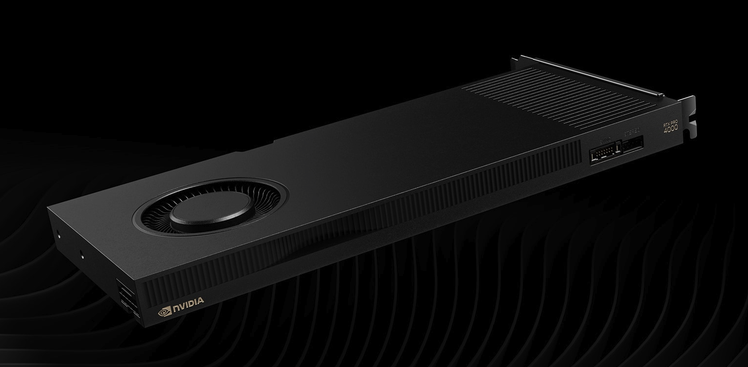
RTX PRO 4000 24 GB VRAM ≈ €2,500 per GPU
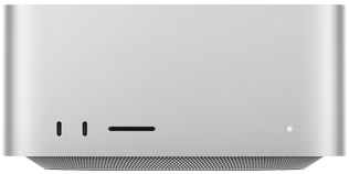
Mac Studio 36–512 GB Unified from €2,999
Ambitious Consumer
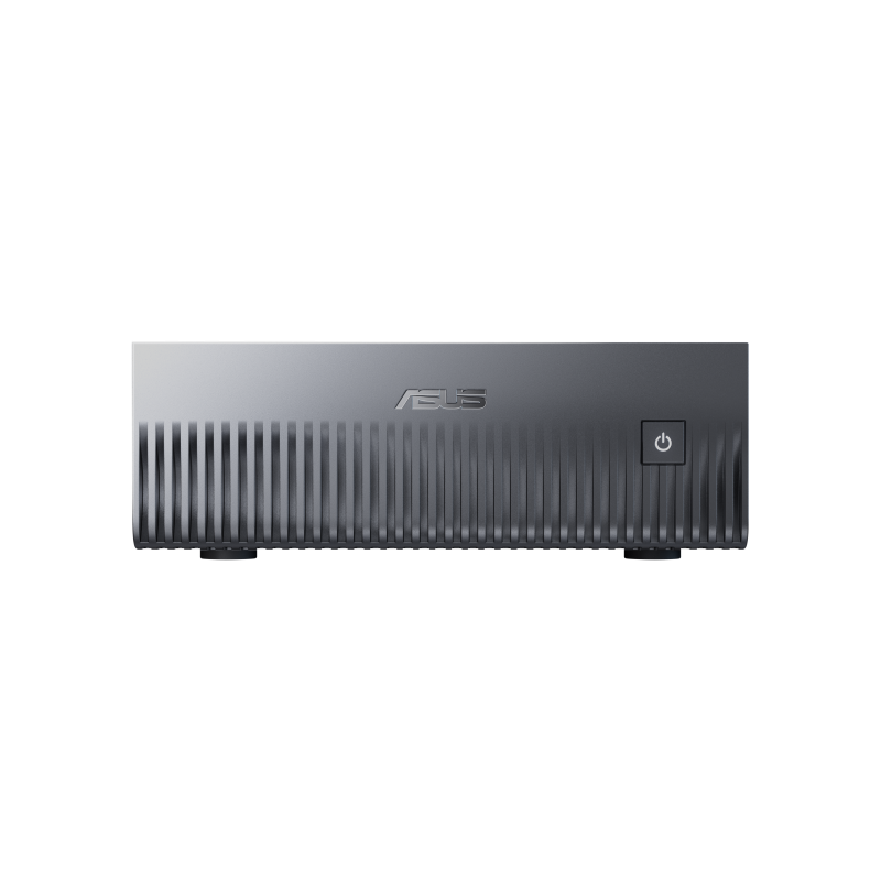
ASUS Ascent GX10
128 GB Unified Memory
≈ €4,850 per system
Enterprise
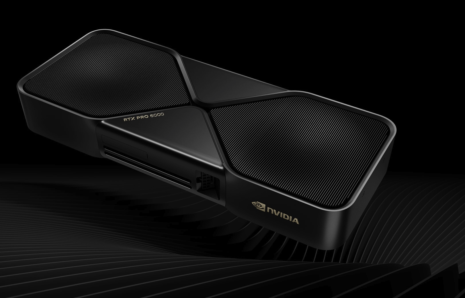
RTX PRO 6000 Blackwell
96 GB VRAM per GPU
≈ €17,700 each
Example configurations — not endorsements or product recommendations.
17
These examples show practical local-inference options rather than a complete buying guide. The consumer column deliberately contains two different approaches. NVIDIA's RTX PRO 4000 Blackwell is a discrete GPU with 24 GB of GDDR7 VRAM and 672 GB/s of memory bandwidth. Twenty-four gigabytes is a useful starting point for quantized coding models, although the usable model size also depends on the context and KV cache. The RTX PRO name belongs to NVIDIA's professional range; consumer here describes the size of the local setup, not NVIDIA's market category. Austrian retail listings put the card at roughly €2,500. This buys the GPU, not a complete computer.
A Mac Studio is the integrated alternative. Apple's current configurations use M5 Max or M5 Ultra and range from 36 GB to 512 GB of unified memory. The 512 GB figure is a configurable maximum, not the base configuration. M5 Max configurations span 36 to 128 GB. M5 Ultra configurations span 96 to 512 GB. Apple starts the M5 Max system at €2,999 and the M5 Ultra system at €6,599 in Austria. Apple says the 512 GB option will become available at the end of October 2026, and the final price of that option is not yet shown. Unified memory is shared by CPU and GPU, so it is not directly equivalent to dedicated VRAM, but the larger configurations can keep very large quantized models in memory. The wide range is important: Mac Studio is one product family, not one fixed capacity.
The middle class is the ASUS Ascent GX10. Its NVIDIA GB10 Grace Blackwell Superchip uses 128 GB of coherent unified LPDDR5x memory. This gives a single developer far more model capacity than a 24 GB graphics card, although its 273 GB/s memory bandwidth is lower than the bandwidth of high-end discrete GPUs. Current Austrian retail listings start near €4,850 for the 1 TB system. ASUS originally announced a €3,499 recommended price, so availability and street pricing matter.
The enterprise class uses RTX PRO 6000 Blackwell GPUs. Each GPU provides 96 GB of GDDR7 ECC memory. Austrian retail listings for the NVIDIA Workstation Edition currently start around €17,700 per card. The three cards in the picture would therefore represent more than €50,000 in GPUs alone. A workstation can contain several cards. Multiple GPUs add capacity and throughput, but one model does not automatically see them as one simple memory pool. The inference runtime must split or replicate the model, and interconnect bandwidth matters. All prices on the slide are rounded snapshots checked on 7 September 2026 and can change. Transition: move from physical machines to the model sizes and deployment classes they can support.
Sources: https://www.nvidia.com/en-us/products/workstations/professional-desktop-gpus/rtx-pro-4000/ ; https://geizhals.at/nvidia-rtx-pro-4000-blackwell-900-5g147-2570-000-a3488409.html ; https://www.apple.com/at/newsroom/2026/08/apple-introduces-new-mac-studio-with-m5-max-and-m5-ultra/ ; https://www.apple.com/at/mac-studio/specs/ ; https://www.asus.com/networking-iot-servers/desktop-ai-supercomputer/ultra-small-ai-supercomputers/asus-ascent-gx10/ ; https://www.idealo.at/preisvergleich/OffersOfProduct/208466423_-ascent-gx10-asus.html ; https://www.nvidia.com/en-us/products/workstations/professional-desktop-gpus/rtx-pro-6000-family/ ; https://geizhals.at/nvidia-rtx-pro-6000-blackwell-workstation-edition-900-5g144-2500-000-a3476784.html
Image sources: RTX PRO 4000 and RTX PRO 6000 images supplied by the presenter; https://www.apple.com/v/mac-studio/specs/b/images/specs/hero__d0yd117u6qy6_large_2x.jpg ; https://dlcdnwebimgs.asus.com/gain/c66958f8-57de-4563-b0db-bd317bfaf1f3/w800
Deployment envelopes
Model Size by Deployment Class
Total parameters log scale
10T
1T
100B
10B
1B
Gemma 4 E2B 5.1B total
Gemini Nano ≈2–4B
Browser / embedded Models run inside the browser
Gemma 4 12B 11.95B total
Qwen3-Coder 30B-A3B 30.5B total
24 GB class Consumer GPU or laptop
Nemotron 3 Super 120B total
Qwen3.8 Flash Next 180B total
128 GB class 4-bit workstation or DGX Spark
DeepSeek V4 Flash 284B total
GLM-5.3 753B total
Kimi K3 2.8T total
Open-weight datacenter Multi-accelerator systems
Gemini ≈3.0T estimate
GPT-6 ≈3.8T estimate
Grok ≈3.9T estimate
Claude Fable ≈6T estimate
Closed frontier Provider-hosted models
Deployment class
Closed-model values are estimates from public benchmark data [1][2], not disclosed parameter counts. Typical error ≈2×.
18
Read the chart from left to right. The horizontal axis shows five practical deployment classes. The vertical axis is logarithmic: every major step represents ten times as many total parameters. This keeps models from 3 billion to several trillion readable on one slide. It also means the visual distance represents a ratio, not a simple difference.
Gemma 4 E2B and Gemini Nano illustrate two different ways a small model can reach a device. Gemma 4 E2B is an open-weight checkpoint with 2.3B effective parameters and 5.1B total when its per-layer embeddings are counted. The chart uses 5.1B because its vertical axis is total parameters. The E in E2B means effective, not total.
Google's original Gemini 1 report disclosed two Nano models with 1.8B and 3.25B parameters, both quantized to 4 bits for deployment. Current Chrome documentation describes hardware-selected variants around 2B and 4B, so the slide shows those rounded current values. Chrome may download the larger or smaller variant after measuring the device. The exact installed variant can change with browser updates and can be inspected at chrome://on-device-internals.
Downloaded does not mean open weights. Chrome downloads, updates and removes the model as a browser-managed component. A web application uses it through the Prompt API and does not receive the weight files as a model it can redistribute, inspect or run in another inference engine. Google separately calls Gemma its open-model family. Gemini Nano is local and downloadable, but it is not an open-weight model in the same sense as Gemma, Llama or Qwen.
Gemma 4 12B has 11.95B parameters and Google positions it for laptops, desktops and small servers. Qwen3-Coder 30B-A3B can fit the 24 GB class when strongly quantized. Its native context is 262,144 tokens, but a 24 GB machine will normally require a shorter practical context because the KV cache also needs memory.
The 128 GB class deliberately shows only two examples. NVIDIA Nemotron 3 Super has 120B total and 12B active parameters with up to 1M context. Its NVFP4 checkpoint targets Blackwell hardware, which makes it relevant to a DGX Spark class machine.
Qwen3.8-Flash-Next is the tightest fit in this group. Hugging Face reports 180B total parameters: a 125B language model with 6B active parameters, plus 51B n-gram embeddings and 4B multi-token-prediction parameters. A simple 4-bit estimate puts the weights near 90 GB before runtime overhead. It supports 262,144 tokens natively, but a 128 GB machine must shorten the practical context or use cache quantization so the weights, KV cache and runtime fit together. This is why the column says 4-bit candidates rather than guaranteed configurations.
DeepSeek V4 Flash has 284B total parameters and activates 13B for each token. GLM-5.3 has 753B total parameters. Kimi K3 has 2.8 trillion total parameters and activates 104B per token.
The providers do not disclose parameter counts for Claude Fable 5.1, GPT-6 Astra, Grok 4.6 or Gemini 3.8 Flash. The plotted figures are our calculations, not vendor claims and not published parameter counts. We use the public Frontier Parameter Model [1]. It predicts parameter-equivalent scale from known-size checkpoints, release date and the Artificial Analysis Intelligence Index, with Kimi K3's disclosed 2.78T size as an anchor. The exact published Artificial Analysis branch is P = 2.780T × 10^(0.045205959 × (AA − 57.112339) − 0.350927951 × age in years). Using the available scores and release dates gives 6.12T for Fable 5.1, 3.82T for Astra, 3.93T for Grok 4.6 from AA 61 and its August 12 release, and 3.04T for Gemini 3.8 Flash from AA 59 and its September 2 release. The slide rounds these values.
This method does not recover literal proprietary weights or reveal architecture and active-parameter counts. The estimator's backtests report median row-level error close to 2× and a conservative factor of about 3× for a new developer [3]. Grok 4.6 builds on Grok 4.5, and Gemini 3.8 Flash is designed for speed and cost efficiency; post-training and serving choices can improve capability without a proportional increase in weights. Treat the four numbers as a common plotting convention for comparison, not hardware-sizing figures.
Sources: Gemma 4 E2B size and terminology: https://ai.google.dev/gemma/docs/core/model_card_4 ; https://huggingface.co/google/gemma-4-E2B ; Gemini Nano sizes and deployment: https://deepmind.google/gemini/gemini_1_report.pdf ; https://developer.chrome.com/docs/ai/understand-built-in-model-management ; https://developer.chrome.com/docs/ai/get-started ; open-model distinction: https://ai.google.dev/ ; 128 GB examples: https://huggingface.co/nvidia/NVIDIA-Nemotron-3-Super-120B-A12B-NVFP4 ; https://huggingface.co/Qwen/Qwen3.8-Flash-Next ; [1] https://github.com/anpaure/frontier-model-sizes#live-factor-models ; [2] Artificial Analysis scores: https://artificialanalysis.ai/models/ , https://artificialanalysis.ai/articles/grok-4-6-benchmarks-and-analysis/ , https://artificialanalysis.ai/articles/gemini-3-8-flash ; [3] https://github.com/anpaure/frontier-model-sizes/blob/main/MODEL_READINESS.md#precision ; official model pages: https://x.ai/news/grok-4-6 ; https://blog.google/innovation-and-ai/models-and-research/gemini-models/3-8-flash-and-3-8-flash-cyber/ ; https://openai.com/index/gpt-6-astra/ ; https://www.anthropic.com/claude/fable ; open model cards: https://huggingface.co/google/gemma-4-12B ; https://huggingface.co/Qwen/Qwen3-Coder-30B-A3B-Instruct ; https://huggingface.co/deepseek-ai/DeepSeek-V4-Flash ; https://huggingface.co/zai-org/GLM-5.3 ; https://huggingface.co/moonshotai/Kimi-K3 . Transition: these classes come from overlapping ecosystems.
Gemma 4 Family
Dense Same path for every token Mixture of Experts Router selects experts
Total Parameters
30B 20B 10B 0
E2B 5.1B total Dense
E4B 8B total Dense
26B-A4B 25.2B total MoE
E Core size, excluding large embedding lookup tables
A Parameters selected by the router for each token
19
Gemma 4 is a family, not one model. The vertical scale is linear and represents total parameter count: a 5.1B bar is roughly one sixth the height of a 30.7B bar. Blue and green describe architecture. Blue models are dense, meaning that every token follows the same network path. Green marks the mixture-of-experts model, where a router selects only some experts for each token.
Effective and active sound similar, but they describe different mechanisms. In E2B and E4B, E means effective. These dense models contain large per-layer embedding tables. The tables must be stored, but each token only performs quick lookups in them. Google therefore describes the computational core as 2.3B or 4.5B effective parameters, while the complete stored models contain 5.1B or 8B parameters.
In 26B-A4B, A means active. The complete mixture-of-experts model contains 25.2B parameters. For each token, its router selects eight experts plus one shared expert from 128 experts in each MoE layer, so about 3.8B parameters participate in the computation. All 25.2B parameters still have to fit in memory for fast inference.
The 12B and 31B variants are dense models with 11.95B and 30.7B parameters. All five are multimodal. The E2B and E4B models support 128K context; the 12B, 26B-A4B and 31B models support 256K. Parameter count is only one dimension: quantization, context size and architecture determine the actual memory requirement and speed. Source: Google Gemma 4 model card, https://ai.google.dev/gemma/docs/core/model_card_4 . Transition: compare that range with the much smaller Qwen 3.6 family.
Memory Provisioning
Recommended Fully Served by VRAM
Sizing Criteria Model Size Quantization KV Cache Context Size Operational Memory
20
The recommended target is to keep the complete inference workload in GPU memory. This avoids moving model data between storage, system RAM and VRAM while generating tokens. Start with the model size. Quantization determines how many bytes the stored weights require, plus scales and metadata. The KV cache needs additional memory and grows with the context size. Its exact size also depends on the model architecture, cache precision and batch size. Operational memory covers the inference engine, temporary compute buffers and memory allocator overhead. Leave headroom rather than planning exactly to the advertised VRAM capacity. On systems with unified memory, such as Apple silicon, CPU and GPU share one memory pool, but bandwidth, allocation limits and the operating system still reduce the amount available to the model. Transition: quantization changes the largest part of this calculation, the weight memory.
Quantization Principle
‹ Ⅱ Pause › 0:00.0 / 0:06.4 ↻ Restart
Original Range 0–100
0 100
18
47
83
÷ 10, then round
Quantized Range 0–10
18 2
47 5
83 8
Reconstructed × 10
20 Δ +2
50 Δ +3
80 Δ −3
21
Start with a deliberately simple example. The original values can occupy many positions between 0 and 100. We choose a scale of 10, divide each value by that scale and round to the nearest integer. That maps 18 to 2, 47 to 5 and 83 to 8. We now store one of only eleven integer values instead of a much finer original number. To reconstruct approximate original values, multiply the stored values by the same scale of 10. The results are 20, 50 and 80. Compared with 18, 47 and 83, the signed differences are +2, +3 and −3. This difference is quantization error: information discarded during rounding cannot be recovered exactly. Real model quantization can use different scales and zero points for tensors, channels or groups. Some methods also calibrate against data or treat important weights differently. The animation explains the basic idea, not a specific file format. Transition: translate the number of bits into model weight memory.
Choosing a Quantization Level
Quality higher fidelity
Memory and File Size smaller larger
Local Sweet Spot
Q2 emergency fit
Q3 tight memory
Q4 default start
Q5/6 conservative
Q8 near reference
BF16 reference size
Practical Rule Start at Q4. Move up if quality breaks.
22
Read this as a practical direction, not a universal benchmark curve. Moving from Q2 toward Q8 or BF16 usually increases file size and memory use while preserving more of the reference model's behavior. The exact quality difference depends on the model, the quantization algorithm, the dataset used for calibration, the runtime and the task. Labels such as Q4 or Q5 are families of formats rather than one standard method. A good local starting point is often a well-supported Q4 quantization. Move to Q5 or Q6 when the model fits comfortably and your evaluation finds meaningful quality loss. Move below Q4 only when memory capacity prevents the model from running, because aggressive quantization can damage reasoning and coding reliability. Q8 often stays close to the reference behavior but saves much less memory than Q4. BF16 represents the high-precision reference here. Always qualify the exact model file, not the label alone. Transition: video codecs show how compression methods can improve across generations.
Video Compression Over Time
1993 MPEG-1 ≈ 600 MB 1995 MPEG-2 / H.262 ≈ 300 MB 2003 H.264 / AVC ≈ 150 MB 2013 H.265 / HEVC ≈ 75 MB 2018 AV1 ≈ 60 MB 2020 H.266 / VVC ≈ 38 MB
23
The repeated image is deliberate. We compare how much data is needed for roughly the same perceived result, rather than showing a sequence of better pictures. The file sizes form an illustrative one-minute 1080p example. They use a simple bitrate scale of 80 megabits per second for MPEG-1, 40 for MPEG-2, 20 for H.264, 10 for HEVC, 8 for AV1 and 5 for VVC. File size equals bitrate multiplied by sixty seconds and divided by eight. That gives about 600, 300, 150, 75, 60 and 37.5 megabytes. These are not measurements from one universal benchmark. MPEG-1 was designed for Video CD-era CIF or SIF resolution, so its 1080p figure is a conceptual extrapolation. The later values make the documented generational improvements easy to see. H.264 can deliver comparable quality at roughly half the bitrate of MPEG-2. HEVC targets another reduction of about half. AV1 arrived in 2018 as an open, royalty-free codec and practical tests show substantial savings over H.264 and VP9. VVC targets about half the bitrate of HEVC. Actual sizes vary with the content, encoder implementation, profile, settings and quality target. Newer codecs can also require more computation. This is the analogy to model quantization: better algorithms can preserve more useful quality within a smaller representation. It does not prove that every newer quantization method or every quantized model is better. We still have to test the exact artifact on our tasks. Sources: MPEG-1 Video, published in 1993, https://mpeg.chiariglione.org/standards/mpeg-1/video.html; ITU-T H.262, July 1995, https://www.itu.int/rec/T-REC-H.262-199507-S/en; ITU-T H.264, May 2003, https://www.itu.int/rec/T-REC-H.264-200305-P; ITU HEVC announcement, January 2013, https://www.itu.int/net/pressoffice/press_releases/2013/01.aspx; AOMedia AV1 specification release, March 2018, https://aomedia.org/press%20releases/the-alliance-for-open-media-kickstarts-video-innovation-era-with-av1-release/; Meta AV1 comparison, April 2018, https://engineering.fb.com/2018/04/10/video-engineering/av1-beats-x264-and-libvpx-vp9-in-practical-use-case/; Fraunhofer HHI VVC overview, finalized July 2020, https://www.hhi.fraunhofer.de/en/departments/vca/technologies-and-solutions/h266-vvc/vvc-overview.html. Transition: next, see how inference uses compute and memory during prefill and decoding.
Prefill and Decoding without KV Cache
‹ Ⅱ Pause › 0:00.0 / 0:18.5 ↻ Restart
Prefill Compute-Bound
Decode Recomputes the Entire Context
User Input Tool Response Thinking
Please build a tested component
with our existing signal store
and add the backend integration
Predicted Token return the final result
return the final
Input return the final
24
This first animation deliberately assumes that no KV cache exists. During prefill, the complete input passes through every transformer layer and the model predicts the first new token. The generated token then joins the input. Without cached keys and values, the next prediction requires another forward pass over the complete sequence. The animation moves the full, growing sequence through one layer at a time. Only after the complete sequence has passed through all layers can the model produce the next token. The model parameters do not move into the model with every step. They remain loaded in memory and the computation reads them again for each pass. Reprocessing the whole context makes uncached generation increasingly expensive as the sequence grows. Transition: the KV cache avoids most of that repeated work.
KV Cache During Inference
‹ Ⅱ Pause › 0:00.0 / 0:12.5 ↻ Restart
Prefill Builds the Cache
Decode Reuses the Cache
User Input Tool Response Thinking KV Cache
Please build a tested component
with our existing signal store
and add the backend integration
Predicted Token return the final result
return the final
Input return the final
25
KV means key-value. The border is a conceptual aid: the cache does not store these token labels. During prefill, every transformer layer computes key and value tensors for the input tokens and stores them in the KV cache. During decode, the model adds key and value tensors for each new token. It reuses the cached tensors instead of recomputing the complete preceding sequence for every prediction. That reuse makes autoregressive decoding practical. The cache still grows with the token count, the number of layers, the attention shape, the batch size and the cache precision. It can consume a substantial amount of VRAM at long context sizes. Transition: apply these components to two concrete Gemma 4 memory plans.
Gemma 4 26B-A4B Memory Provisioning IT QAT UD-Q4_K_XL by unsloth · 3.8B active / 25.2B total · one inference slot · F16 KV cache
Model Size KV Cache Runtime
Memory in VRAM / Unified Memory (GiB)
0 4 8 12 16 20 22
16.72 GiB 13.27 GiB Model
1.45 GiB KV
2 GiB Runtime
64K 17.97 GiB 13.27 GiB Model
2.70 GiB KV
2 GiB Runtime
128K 20.47 GiB 13.27 GiB Model
5.20 GiB KV
2 GiB Runtime
256K
Context Size
All 25.2B parameters must fit in memory. Totals use a 2 GiB runtime reserve.
26
This is a planning estimate for the quantized Gemma 4 26B-A4B artifact shown in the reference. The weight file remains constant at 13.27 GiB for every context size. A4B means that about 3.8 billion of roughly 25.2 billion total parameters are active for a token. That can reduce compute, but it does not turn the model into a 4B memory footprint. All expert weights still have to reside in memory. The F16 KV cache grows from 1.45 GiB at 64K to 2.70 GiB at 128K and 5.20 GiB at 256K. The runtime estimate is a range of one to two GiB. The totals shown here use the conservative two GiB endpoint: 16.72, 17.97 and 20.47 GiB. These numbers plan capacity; the actual allocation depends on the runtime, backend, batch settings and model file. Read the startup logs before treating the fit as guaranteed. Transition: compare this mixture-of-experts model with the dense Gemma 4 12B.
Qwen 3.8 27B Memory Provisioning UD-Q4_K_XL by unsloth · 27B dense · 16 KV layers · one inference slot · F16 KV cache
Model Size KV Cache Runtime
Memory in VRAM / Unified Memory (GiB)
0 6 12 18 24 30 36
22.39 GiB 16.39 GiB Model
4.00 GiB KV
2 GiB Runtime
64K 26.39 GiB 16.39 GiB Model
8.00 GiB KV
2 GiB Runtime
128K 34.39 GiB 16.39 GiB Model
16.00 GiB KV
2 GiB Runtime
256K
Context Size
Hybrid architecture: 16 of 64 layers grow the KV cache. Totals use a 2 GiB runtime reserve.
27
This planning estimate uses the 17.6 GB decimal UD-Q4_K_XL artifact published by unsloth, which is 16.39 GiB. Qwen 3.8 27B has 64 layers, with 16 full-attention layers, four KV heads and a head dimension of 256. With F16 keys and values, the growing KV cache is 4 GiB at 64K, 8 GiB at 128K and 16 GiB at the native 256K context. Adding a two GiB runtime reserve produces planning totals of 22.39, 26.39 and 34.39 GiB. The vision projector is not included. Actual llama.cpp allocation, state checkpoints and batch settings can require more headroom. Sources: https://huggingface.co/unsloth/Qwen3.8-27B-GGUF/blob/main/Qwen3.8-27B-UD-Q4_K_XL.gguf ; https://huggingface.co/Qwen/Qwen3.8-27B ; https://huggingface.co/Qwen/Qwen3.8-27B/blob/main/config.json . Transition: hardware capacity is only one part of the decision. The next chapter asks how we control quality.
Quality: Loop / Graph Engineering
LOCAL MODELS
FOR AI-ASSISTED
CODING
01
WHY
Why local models?
02
HOW
llama.cpp + Gemma 4
03
SHOW
Capstone
04
CHALLENGES
Speed and quality
SPEED
Hardware requirements
QUALITY
Loop / graph engineering
28
Open the second practical challenge: quality. The model will make mistakes, so the surrounding workflow has to evaluate its output and remain in control. Begin with Claude's goal-review workflow, then show how bounded model sessions, deterministic validation, independent reviewers and fresh repair attempts improve reliability.
The surrounding system
Engineering Around the Model Models make mistakes. The surrounding system must detect them and remain in control.
Bound each model turn and run verification through external tools, so inner loops cannot block the workflow.
A well-structured codebase gives the model reliable patterns to follow.
Application-specific instructions and skills cover Angular, Spring, Playwright, and project conventions.
24/7 local inference makes loop / graph engineering with independent review and repeated validation practical.
29
Do not expect the model to be perfect. It will make mistakes, and the surrounding system must detect those mistakes and remain in control.
First, bound every model turn and run verification outside the model session. Smaller local models can start their own verification, repeat checks indefinitely and never return control. When that happens, the outer agent loop cannot continue. External tools such as builds, tests and browser checks provide an independent result while the orchestrating workflow decides whether to continue.
Second, begin with a well-structured codebase. The model learns from the application in front of it. Clear architecture, consistent conventions and good existing code give it reliable patterns to copy.
Third, encode knowledge about the actual application in instructions and reusable skills. Generic Angular guidance is only the beginning. The agent also needs the project's Spring patterns, Playwright conventions and other application-specific rules.
Finally, use the operational advantage of local inference. The model can run continuously, so a workflow may spend more wall-clock time on a task and use independent review agents plus repeated validation. The same number of passes can be harder to justify with frontier models because every pass consumes provider tokens and quota. Structuring the work as bounded model sessions, tools, reviewers and validation steps is loop / graph engineering. Transition: show why continuous local execution makes this approach practical.
A Practical Starting Point
Q4 quantized Gemma 4
+
24 GB VRAM
A usable entry point for local AI-assisted coding
31
This is the practical answer to the title question. Gemma 4 26B-A4B is usable as a local coding model when quantized to the Q4 artifact shown earlier. Our planning estimate puts the model, F16 KV cache and runtime at about 18 GiB for 128K context and 20.5 GiB for 256K context, so 24 GB is the entry hardware class. Actual allocation still depends on the runtime and settings, so check the startup logs. Larger open-weight models, including DeepSeek, remain promising, but they move beyond this entry setup and need more hardware and their own qualification. For a first practical system, start with Gemma 4 and put a controlled agent loop around it.
Thank you
Questions? Local models for AI-assisted coding
Thank the audience. Point to the QR code for feedback at https://soverius.ai/feedback/dc9d7006. The short code is dc9d7006. Leave this final screen visible after questions.



 Claude Code
 llama.cpp
 Gemma 4